
Porto Seguro Challenge – 2nd Place Solution

Adriano Marques
CEO at XNV

We are pleased to announce that we got second place in the Porto Seguro Challenge, a competition organized by the largest insurance company in Brazil. Porto Seguro challenged us to build an algorithm to identify potential buyers of their products. If you are interested in knowing how to do the same and still discover the secrets that led us to second place, read on below!
Introduction
In this problem, Porto Seguro provided us with data of users who bought or did not buy one of its products. The main objective was to optimize telemarketing sales by offering products to those who really need them, and for that, we should build a model that predicts the probability of purchasing a product.
The first curiosity and complication was that all data was anonymized. That is, we cannot say what each field meant besides ID and Target. So we have this bunch of numbers, we have no idea how best to work with each one, and we need to build a machine learning model. How can we improve this situation? Looking better at our data.
Exploratory Data Analysis
Data analysis started with a simple task, understanding basic dataset statistics. We would also like to understand the target distribution of the problem.


From this analysis, we have already been able to extract some interesting information. First, the test dataset is considerably larger than the training dataset, so it’s quite likely that we can explore some techniques like pseudo labeling here. Second, we have several null fields, and they seem to follow some pattern, where several fields have the same number of nulls as others, indicating a possible correlation between these fields when registering the user. Third, the target is unbalanced, with only 20% of users buying a produc
Despite the dataset being anonymized, Porto Seguro gave us essential information, the type of each variable. After some fundamental analysis like histogram and counting, we discovered another critical and strange piece of information. There are several categorical variables with high cardinality. Var4, for example, has more than 13.000 unique values in the training dataset!
With categorical data having so many unique values, it is possible to have data that exists in the test and not in training, especially if we remember that the test dataset is larger than the training dataset. Let’s see which fields present data in the test set and not in the training set.

Here it is. Several fields have test values that do not exist in training. The ID field was left as an example of how the algorithm works, as it is expected to present this behavior.
We performed other analyzes, such as 2D visualization of the solution space and feature importance.


From these graphs, we can expect that some variables will dominate the algorithm’s decision process and the solution space will be easy to reach an X value (predominant yellow region) and the difficulty will be to find mixed buyers in the rest of the space.
We already have much information to work with, and now we need to get our data in a better format to make it easier to train our model.
Pre-processing
Pre-processing our data allows us to leave it in a better format to facilitate training our model, as well as creating other features from what we already have (feature engineering). One of the most important points of our solution was to work with the categorical variables of high cardinality so that they start to make sense. Given this peculiar characteristic, teams that tried to use techniques like One Hot Encoding saw their solution fail. Other types of grouping, such as grouping by rare classes, for example, did not work very well either. We even applied a Variational Auto Encoder to the high-resolution matrix generated by One Hot Encoding, hoping that we would arrive at a similar representation but with far fewer dimensions. Despite a very cool technique, which may have a post about it, it wasn’t the best solution.
The following graph gave us our final idea:
As we can see, the multivariate analysis of this variable with the target indicates that the value of the variable actually matters. Higher values on Var4 are more likely to be a buyer. So how can we group close values together without losing this pattern? First, we scale our variables between 0 and 1, and then we apply round 3 in the decimal digits. By doing this, we reduced it to just 1800 possibilities in variable 4, we maintain this correlation with the target, and most importantly, all data is now mapped between training and testing.

For feature creation, we make all processes parameterizable. This is because we want each model to be trained differently, adding variance to our ensemble. As a possibility of extra features, we added:
- Columns stats – Min, Max, Avg, Std
- NaN Values stats – Count, Avg, Std
- Categorical var – Count
- Nan values imputer – IterativeImputer Sklearn
- Frequency Encoder – var4, var5, var11, var12
- Aggregation by var4 – Mean, Std, Min, Max
- Target Encoding – var4, var6
- Label Encoder – All categorical var
- PCA
- ICA
- Feature Agglomeration
Modeling
As we worked, we tested several different models and approaches, but we’ll only focus here on what worked best. To create our validation set and perform cross-validation, we used a StratifiedKfold with 5 splits. All models and out-of-folds for each split were saved at the end of training.
As already shown, the data is unbalanced and in our methodology we oversampled the training set to calibrate the model by 50% for each target.
Our final ensemble is made up of 3 types of models: LightGBM, XGBoost and CatBoost. All of them have been optimized using Optuna.


We trained a total of 36 models, being 12 LightGBM, 12 XGboost and 12 Catboost. As stated earlier, each model was trained using different preprocessing and feature engineering to add diversity to the model. The experiments were all repeated 10x, changing the split seed and all other random processes in the data processing. This ensured more significant variance and helped to stabilize our validation.
All out-of-folds were collected and analyzed for an ensemble. In total, we had 10x5x36 = 1800 out-of-folds for the ensemble. The next figure shows the heatmap between each of the models. You can see that there is variance between them.
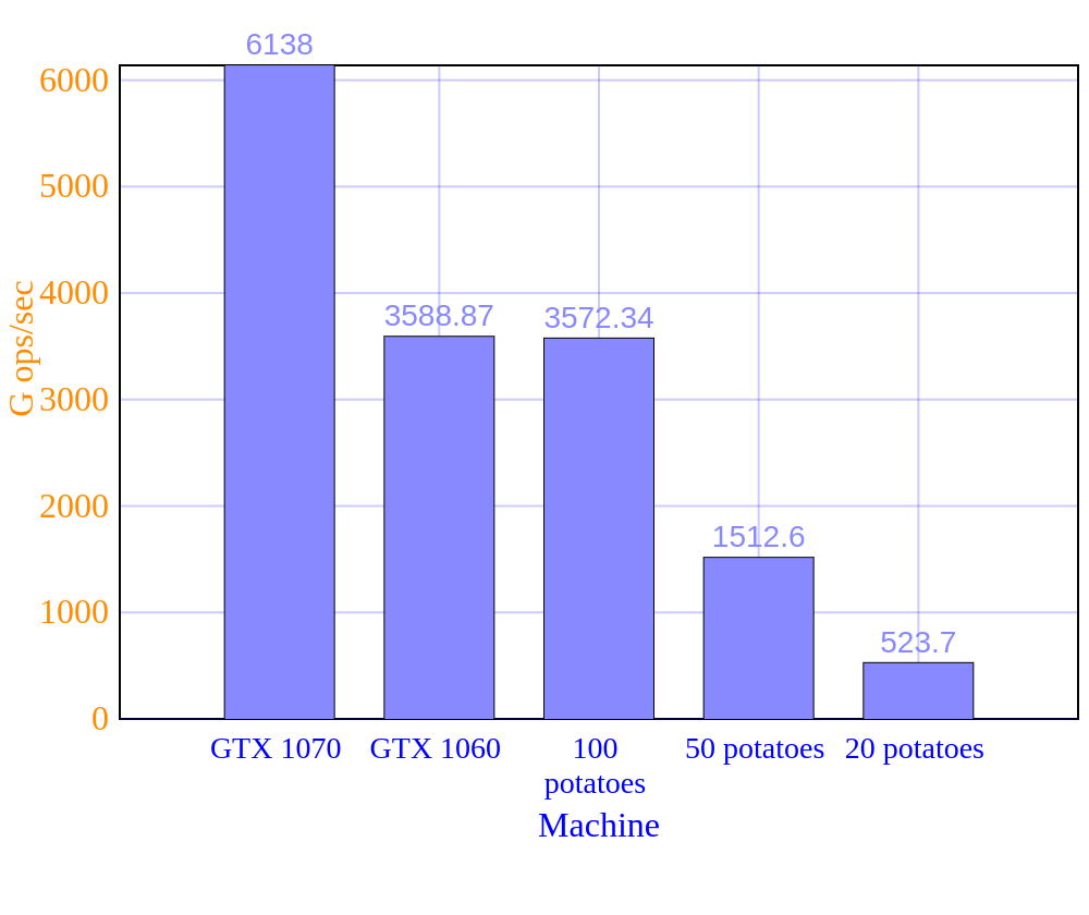
In total, we performed more than 350 experiments, with more than 5000 models being trained. All these processes were performed using the Amalgam cluster, which contains machines with multiple GPUs and a large amount of Ram, which allowed us to train faster and run multiple experiments in parallel. Development was done using python and docker, and all experiments were tracked using Aurum.


Results
Due to time constraints for the end of the competition and daily submission limits (3), we could not test all models in the test set. However, within what we proposed to do and were able to test, this was our best model:
- LigthGBM
- 10 seeds
- StratifiedKfold – 5 splits
- All preprocessing and feature engineering techniques
- CV score: 0.70586
- Public score: 0.69699
- Private score: 0.69557
This model alone would be enough to guarantee us the second position, but we wanted to see the capacity of our ensemble.
- 36 models (12 LGB + 12 XGB + 12 CatB)
- 10 seeds
- StratifiedKfold – 5 splits
- Different preprocessing and feature engineering techniques for each model
- Mean ensemble – average of the probabilities of each out-of-fold
- CV score: 0.69747
- Public score: 0.70420
- Private score: 0.69965

It’s possible to notice that our models are quite robust in terms of validation, and also not overfitted in none of the leaderboards. This was possible thanks to our pre-processing. A deeper analysis of the model’s performance allows us to go to the conclusion of the problem.
Conclusion
This competition presented us with a recurrent and considerably difficult problem, made more complicated by having anonymized variables. We are happy that we have not only solved the problem, but we have achieved second place in terms of scoring and have delivered an end-to-end producible solution.
Our model had a ~70% ability to identify buyers within the available data. Our classification report shows that the model is well calibrated in terms of precision and recall. However, we did it this way because it is a competition, but for a real scenario, a higher recall is preferable in relation to precision. That’s because greater recall ensures greater success in finding positive cases, which is what really matters here.
It is also possible not to work with the binary prediction but with the probability that each user is a buyer. Thus, we can also use this model to create marketing strategies for “almost” buyers, understand what is needed for them to become buyers, and consequently increase sales.
Finally, we would like to emphasize that this is a difficult problem in nature, as the reason a person does not buy a product is not always in the data. This ends up causing noise in the data, as a user may have the same characteristics as a potential buyer, but it is not thanks to external variables that we have no way of knowing. Therefore, it is possible to continue the project using more recent techniques such as noisy student, PU learning, and label smoothing to add uncertainty in label 0 (non-buyer) and perhaps help better converge the model.
THE BLOG
News, lessons, and content from our companies and projects.
41% of small businesses that employ people are operated by women.
We’ve been talking to several startups in the past two weeks! This is a curated list of the top 5 based on the analysis made by our models using the data we collected. This is as fresh as ...


Porto Seguro Challenge – 2nd Place Solution
We are pleased to announce that we got second place in the Porto Seguro Challenge, a competition organized by the largest insurance company in Brazil. Porto Seguro challenged us to build an ...
Adriano Marques
CEO at XNV

Predicting Reading Level of Texts – A Kaggle NLP Competition
Introduction: One of the main fields of AI is Natural Language Processing and its applications in the real world. Here on Amalgam.ai we are building different models to solve some of the problems ...
João Paulo Martins
Data Scientist XNV

Porto Seguro Challenge
Introduction: In the modern world the competition for marketing space is fierce, nowadays every company that wants the slight advantage needs AI to select the best customers and increase the ROI ...
João Paulo Martins
Data Scientist XNV

Sales Development Representative
At Exponential Ventures, we’re working to solve big problems with exponential technologies such as Artificial Intelligence, Quantum Computing, Digital Fabrication, Human-Machine ...

Rodolfo Egarter
COO @ Pluo

Exponential Hiring Process
The hiring process is a fundamental part of any company, it is the first contact of the professional with the culture and a great display of how things work internally. At Exponential Ventures it ...
Rodolfo Egarter
COO @ Pluo

Exponential Ventures annonce l’acquisition de PyJobs, FrontJobs et RecrutaDev
Fondé en 2017, PyJobs est devenu l’un des sites d’emploi les plus populaires du Brésil pour la communauté Python. Malgré sa croissance agressive au cours de la dernière année, ...
Adriano Marques
CEO at XNV

Exponential Ventures announces the acquisition of PyJobs, FrontJobs, and RecrutaDev
Founded in 2017, PyJobs has become one of Brazil’s most popular job boards for the Python community. Despite its aggressive growth in the past year, PyJobs retained its community-oriented ...
Adriano Marques
CEO at XNV

Sales Executive
At Exponential Ventures, we’re working to solve big problems with exponential technologies such as Artificial Intelligence, Quantum Computing, Digital Fabrication, Human-Machine ...
Rodolfo Egarter
COO @ Pluo

What is a Startup Studio?
Spoiler: it is NOT an Incubator or Accelerator I have probably interviewed a few hundred professionals in my career as an Entrepreneur. After breaking the ice, one of the first things I do is ask ...
Adriano Marques
CEO at XNV

Social Media
At Exponential Ventures, we’re working to solve big problems with exponential technologies such as Artificial Intelligence, Quantum Computing, Digital Fabrication, Human-Machine ...
Rodolfo Egarter
COO @ Pluo

Hunting for Unicorns
Everybody loves unicorns, right? But perhaps no one loves them more than tech companies. When hiring for a professional, we have an ideal vision of who we are looking for. A professional with X ...
Rodolfo Egarter
COO @ Pluo
Stay In The Loop!
Receive updates and news about XNV and our child companies. Don't worry, we don't SPAM. Ever.
